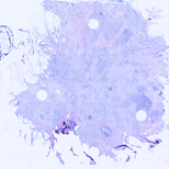
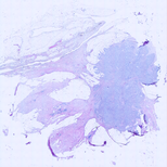
HER2 FFPE-smFISH was repeated in the four cases indicated for which additional tissue sections could be retrieved. After imaging HER2 mRNAs (black dots) and DAPI-stained nuclei (not shown) at 100X magnification in multiple fields of view (black squares), the same tissue section was washed, re-stained with Hoechst 33342, and then fully scanned at 40X (images not shown). After this, once again the same tissue section was washed, re-stained with hematoxylin-eosin (H&E), and then scanned at 10X. As described in Materials and Methods, we used the information contained in the 40X DAPI scan to register the position of each 100X smFISH image on top of the 10X H&E scan, finally obtaining the composite images shown here. To zoom-in a case, click either the image or the case number below. In case #18, the individual fields of view used to build the full H&E image are clearly distinguishable due to illumination variations across different parts of the same field (this is an intrinsic property of the optics in our scanning system. This, however, does not at all affect the accuracy of the image registration process, and could be easily filtered out computationally). As it can be appreciated, almost all of the 100X fields of view where smFISH signals were imaged – and which were selected based on the location of tumor regions annotated by a pathologist on an adjacent or close-by tissue section stained by H&E – indeed fall inside regions with a high density of malignant cells. This confirms the validity of the approach described in the paper to select the positions for smFISH signal acquisition. Importantly, this approach provides the first example of integration between FFPE-smFISH and digital pathology, setting the stage for many future applications of this powerful quantitative technique in diagnostics.

Click to open full size images.

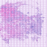
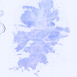
For each case, we arranged all the z-projections of the DAPI images acquired at different locations inside each case inside a 9x9 matrix plot (thus, adjacent images should not be considered as coming from the same location in the tissue section, but arbitrarily stitched together). The fact that the matrix plots are not completely filled is due to the fact that typically less than 81 fields of view were imaged in each case. The number below each matrix corresponds to the sample ID described in Supplementary Table S3. To visualize each case at higher magnification, click on the matrix plot of interest, then use the large navigation panel appearing below all the cases. Use the menu at the bottom of the page to select which feature to show on top of the DAPI z- projection. The following features can be visualized: position of all the HER2 (cyan dots) or ER (red dots) mRNA molecules detected in the field of view; boundary of the manually segmented nuclei (blue polygons) [note: if the case was not segmented, this feature will not be displayed]; boundary of the regions in the image where cells are located (green). The green ticks point to the area without cells, whereas the area on the opposite side of the green boundary contains cells. To speed up the visualization, the features are displayed only on top of the field of view that is currently in the center of the navigation panel.

Click images to open below.

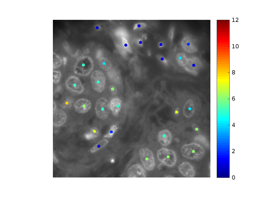
First, select the desired case, the transcript to visualize (HER2 or ER) and a field of view using the drop-down menu displayed on top of the page. A z-projection of DAPI with color-coded dots in the center of manually segmented cells will then appear. The color bar on the right indicates the transcript density ranked on a scale from 0 (lowest) to 10 (highest). The ranking was obtained by binning all the transcript density values in 10 different bins spanning from 0 to 0.5 mRNAs/μm³. The relative frequency of each bin is shown in the histograms in Figures 3A and 3B.

Sample: Image: ER HER2